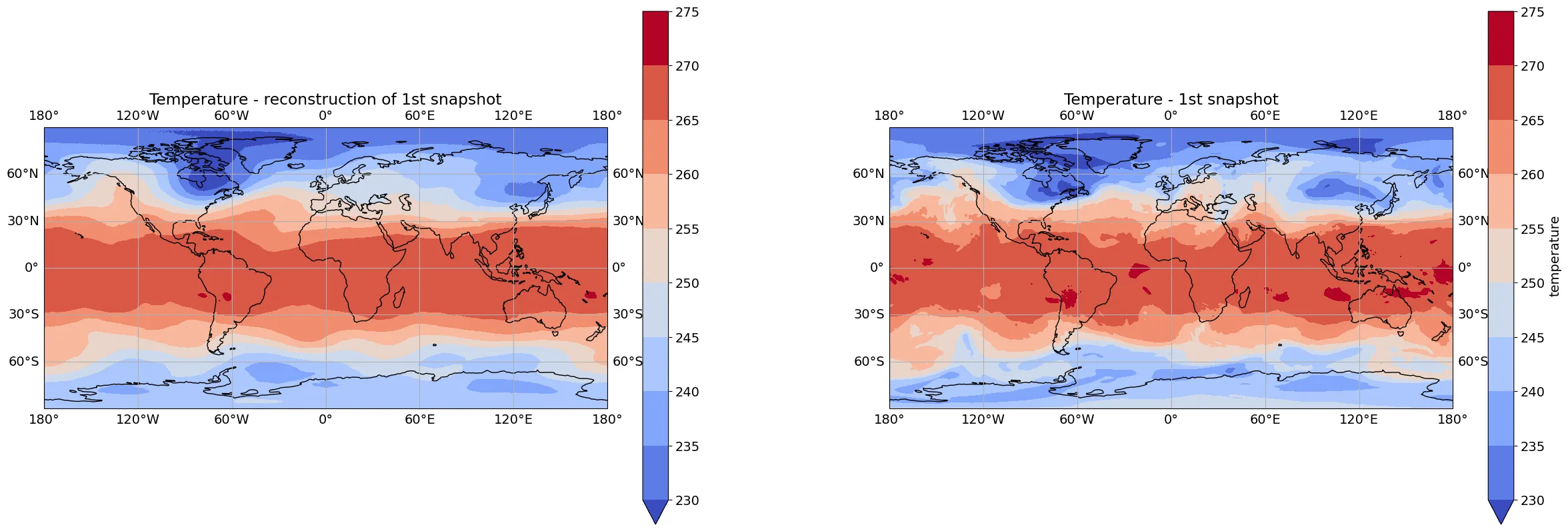
The image above is not a decorative matrix. It is the result of running SVD-ROM on a global atmospheric dataset: a reduced reconstruction on the left and the original temperature field on the right. The broad structure survives; fine-grained variation is smoothed away. That trade-off is the project in one picture.
The dataset behind the image
The demonstration uses an approximately 17 GiB slice of ERA5 reanalysis data: 4,380 atmospheric-temperature snapshots on a 721 × 1,440 latitude–longitude grid at 500 hPa. Flattened for decomposition, each snapshot contains more than one million spatial samples.
A conventional in-memory workflow makes this scale awkward on a personal computer. SVD-ROM keeps the array chunked with Dask and labelled with Xarray, so preprocessing, decomposition, inspection and reconstruction can remain in one scientific workflow.
What thirty components retain
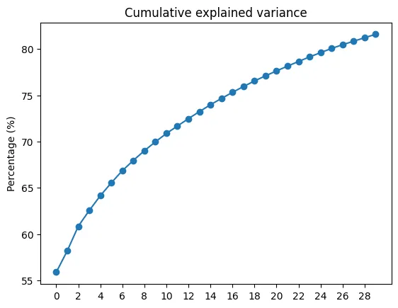
Figure 01 Cumulative explained variance for the ERA5 demonstration. Thirty components retain a little over 80% of the variance; the first component alone accounts for roughly 56%.
The source matrix has 4,380 temporal columns. The demonstration retains thirty components, giving a reported compression ratio of 145. This is deliberately not lossless compression: the aim is to preserve dominant behaviour in a representation small enough to analyse, compare and use in downstream reduced-order models.
The cover shows the consequence. Large-scale temperature bands and continental patterns remain legible, while local detail becomes smoother. Keeping more components would improve the reconstruction at the cost of a larger model.
Choosing a decomposition that fits the machine
SVD-ROM exposes both TSQR and randomized SVD paths through Dask. On a smaller, approximately 8.4 GiB ERA5 slice, the leading singular values from the two methods are almost identical; the approximation begins to diverge only among the smaller components.
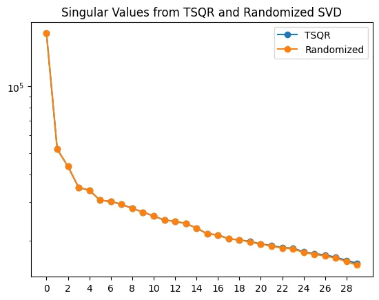
Figure 02 Leading singular values from TSQR and randomized SVD. Their agreement matters because the randomized route is substantially easier on memory for this shape of data.
That comparison captures an important engineering decision. A mathematically valid algorithm is not necessarily a practical one when the intermediate arrays exhaust local memory. Chunk layout, rechunking, lazy execution and the shape of the matrix are part of the numerical method, not infrastructure details to be hidden after the fact.
The modes remain scientifically interpretable
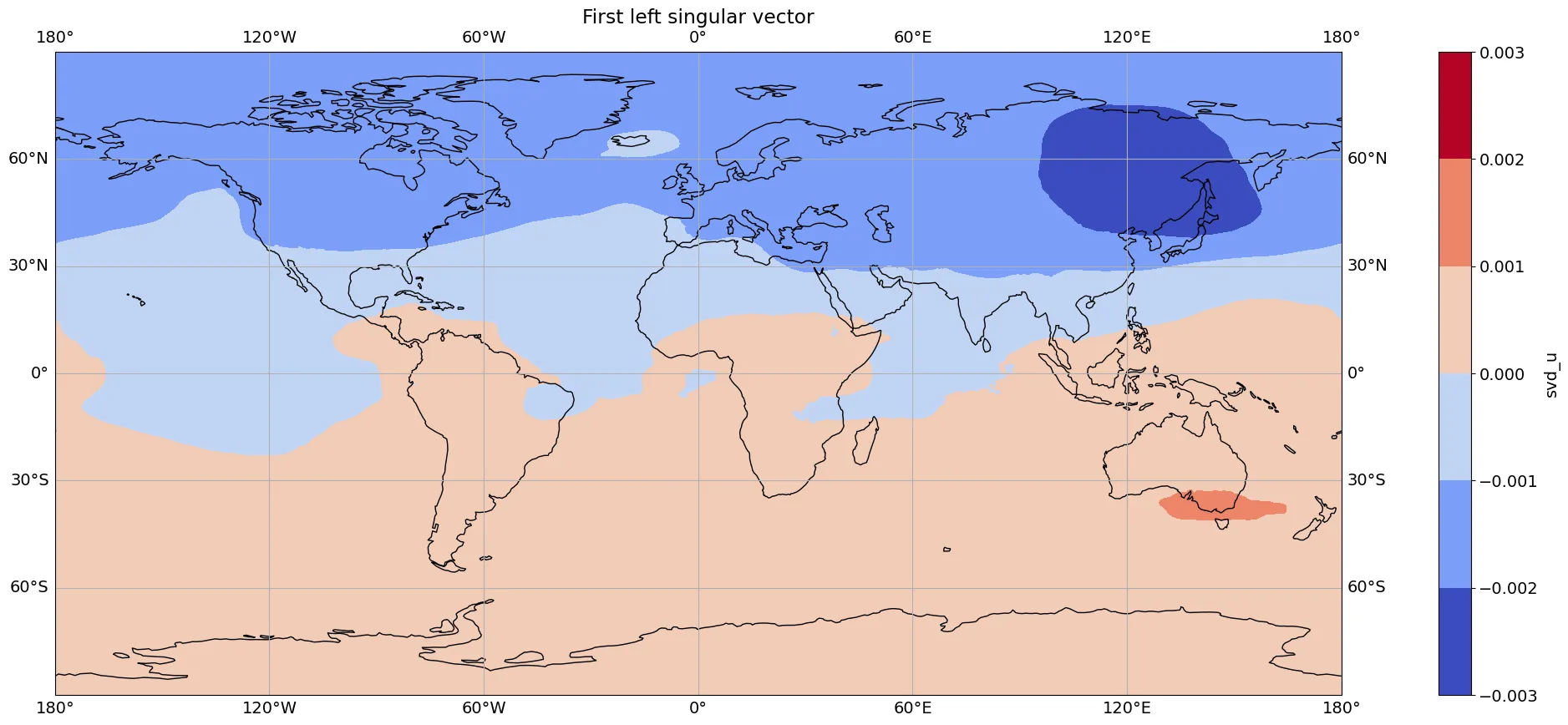
Figure 03 The first spatial SVD mode. Its north–south structure pairs with a strongly annual temporal component, recovering the dominant seasonal temperature cycle.
Because the package carries Xarray coordinates through the calculation, a singular vector can be returned to its latitude–longitude geometry instead of remaining an anonymous column of numbers. Here the first spatial mode separates correlated temperature variation across the Northern and Southern hemispheres; its corresponding temporal vector oscillates annually.
This is why reduced-order modelling is more than making an array smaller. The decomposition can expose coherent spatial and temporal structures that are difficult to see in millions of raw values.
What the library is for
The same SVD foundation supports techniques such as Principal Component Analysis, Proper Orthogonal Decomposition and Dynamic Mode Decomposition. The repository includes progressively larger demonstrations, including decomposition and forecasting experiments on ERA5 data.
SVD-ROM remains active open-source work. The current goal is a library whose scaling behaviour is explicit, whose outputs retain scientific metadata, and whose numerical choices can be inspected rather than accepted as a black box.
Reduce the computation without erasing the structure that made the data worth studying.